


XAFS Data Processing III. – Normalization
The data in this demo was collected by RapidXAFS
XAFS data is essentially the relationship between the absorption coefficient and energy of the sample for X-rays, and the strength of the absorption coefficient is not only related to energy, but also related to the thickness of the sample, test conditions (such as luminous flux, etc.). Therefore, it is not advisable to directly compare the XAFS data of the two sets of samples, as shown in the figure below, directly comparing the m(E) curves, the noise and signal of the two data are not at the same level, resulting in a visual comparison:

Therefore, it is necessary to use the normalization method to deduct the front edge and classify the distance between the front and back of the edge as 1, which is normalization. It is relatively easy to understand from the following diagram:

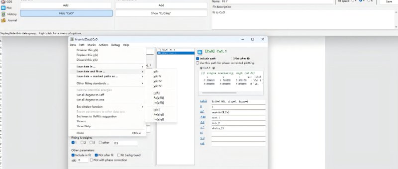
In the normalization process, the normalization module of the Athena software needs to be operated, mainly for the pre-edge and post-edge parts to select points, and a line is determined by two points. First, select the pre-edge line and post-edge line in the paint module, and the corresponding spectral lines will be automatically displayed in the image.

In the normalization process, the normalization module of the Athena software needs to be operated, mainly for the pre-edge and post-edge parts to select points, and a line is determined by two points. First, select the pre-edge line and post-edge line in the paint module, and the corresponding spectral lines will be automatically displayed in the image.
The pre-edge is basically a straight line, as long as the pre-edge line coincides with the data in front of the edge. The focus is on post-edge data normalization, where the post-edge line passes through the center of most of the peaks.

The Normalization order is the number of curves of the post-edge line, where 1 represents 0 times, that is, a horizontal line, 2 represents 1 time, which is a one-time curve, and the curve is completely controlled by two points, and 3 represents 2 times, which is a curve, which is suitable for slightly bending behind the edge. The following diagram shows the case when the normalization order is 1, 2, and 3, respectively.

After the normalization process, select Normalized in the Paint module to display the normalized data.